At SUAS the mapping task sounds simple: fly the field, come back with one picture of it. What you actually come back with is a few hundred overlapping frames shot from a moving, vibrating platform. Turning those into one consistent image is stitching. Turning them into something you can measure on is an orthomosaic. They are not the same thing, and the difference cost me time on our UAS work before I learned to respect it.
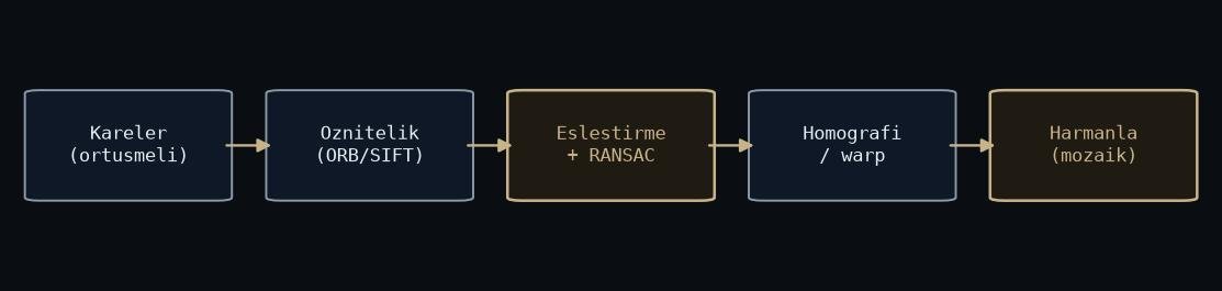
Diagram: my own drawing.
The classical pipeline still works
Stitching two frames is a known recipe: detect keypoints (ORB if you are in a hurry, SIFT if you want robustness), match descriptors, estimate a homography with RANSAC, warp one frame onto the other, blend the seam. OpenCV’s stitching module packages the whole chain, bundle adjustment included, and for a first map it is genuinely good.
What the module actually runs is longer than the two-frame recipe: it matches every pair, keeps the confident ones, estimates the geometry globally instead of chaining frame to frame, compensates exposure gain between images, routes the seam line through the overlap instead of cutting through the middle of an object, and only then blends. Each of those extra steps exists because a real flight violates some assumption of the clean two-frame recipe, and knowing which step absorbs which violation is what lets you debug a bad mosaic instead of staring at it.
The part worth understanding instead of importing: a homography maps a plane to a plane. It is only valid when the scene is planar or the camera purely rotates. Aerial frames from 20 to 40 metres over a flat field are close enough to planar that it works. Fly over buildings or trees and parallax breaks the assumption: things at different heights refuse to agree on one transform, and you get smeared double edges that no blending hides.
And before any of this: undistort. Lens distortion bends the straight lines homographies rely on, and residual distortion accumulates across a strip of frames into a map that slowly curls.
A panorama is not a map
The stitcher output looks great and measures wrong. Scale drifts across the mosaic, and the perspective is whatever your flight happened to be.
An orthomosaic makes a stronger promise: every pixel rendered as if seen from straight above, uniform ground resolution, a real ground coordinate under each pixel. Getting there needs camera poses, bundle adjustment across all frames, and orthorectification against a terrain model. That is photogrammetry, not just stitching. My rule of thumb: if the deliverable is “roughly where is the target”, a stitched map can be enough. If the deliverable is coordinates, build the orthomosaic.
In practice the decision is a checklist, not a debate. What question does the map answer, and who consumes it? If a human looks at it and says “the tent is near the third tree line”, stitched is fine. If a number leaves the map, a coordinate, a distance, an area, then someone will eventually trust that number, and the mosaic has to be built to deserve the trust. We got this wrong once in the direction that hurts: a nice-looking panorama quietly treated as if it were metric.
Overlap decides the outcome before any algorithm runs
RANSAC needs inlier matches, and matches need shared content between frames. Photogrammetry practice is high forward overlap between consecutive frames and generous side overlap between flight lines, and after watching thin overlap produce weak match chains and drifting geometry, I do not argue with it. Grass is the worst case: a texture-poor surface gives you few features exactly where you need them most, so the overlap is your only safety margin.
This rhymes with the tiling rule from the dataset post: overlap is not a tuning knob you sweep later. It is set by the requirement, at planning time, before the algorithm sees a single pixel. Fly boring: constant altitude, camera at nadir, straight parallel lines.
Case study: the SUAS mapping line, from model city to field
For SUAS the map is not the end product, it is the context layer. The detection side of the system looks for mannequins and tents; the mapping side has to answer where on the field each one sits. We flew at 20 to 40 metres with the camera at nadir, and at that altitude a target occupies roughly 80 to 120 pixels in a 4K frame. Small enough that every geometric error in the map translates directly into a localization error on the target.
Before the pipeline ever saw field data, we validated it on a model city: a scale mock-up we could photograph on demand, under controlled light, with a layout we knew by heart. That choice paid for itself quickly. Frame ordering bugs, seam placement, exposure steps between images, all of it surfaced on the model, where a full iteration cost minutes instead of a flight slot. When the stitched model city stopped showing ghosts and curled edges, we knew the line itself was sound, and that any new artifact appearing in the field would come from the flight, not from the code.
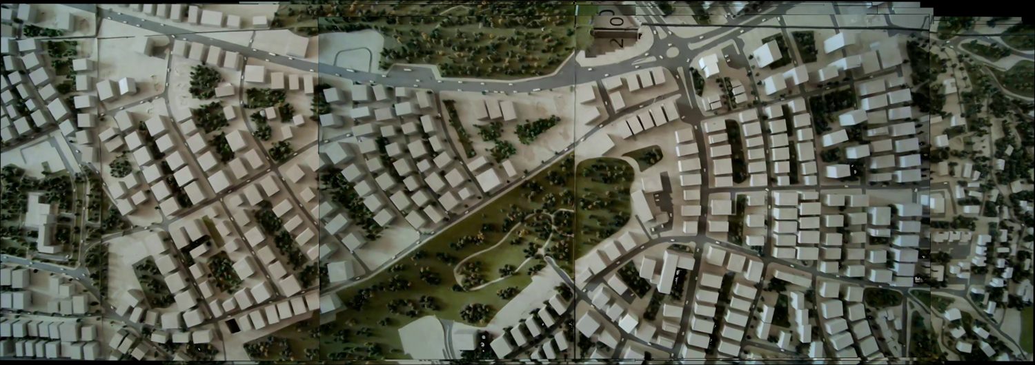
Frame: real output from the project.
The field run followed the boring-flight doctrine from the previous section: constant altitude, straight parallel lines, generous overlap. The result is the orthomosaic below. The difference from the model city run was exactly the list of failure modes in the next section: wind nudging the platform off its line, light changing mid-flight, and real grass giving far fewer features than painted cardboard ever did.
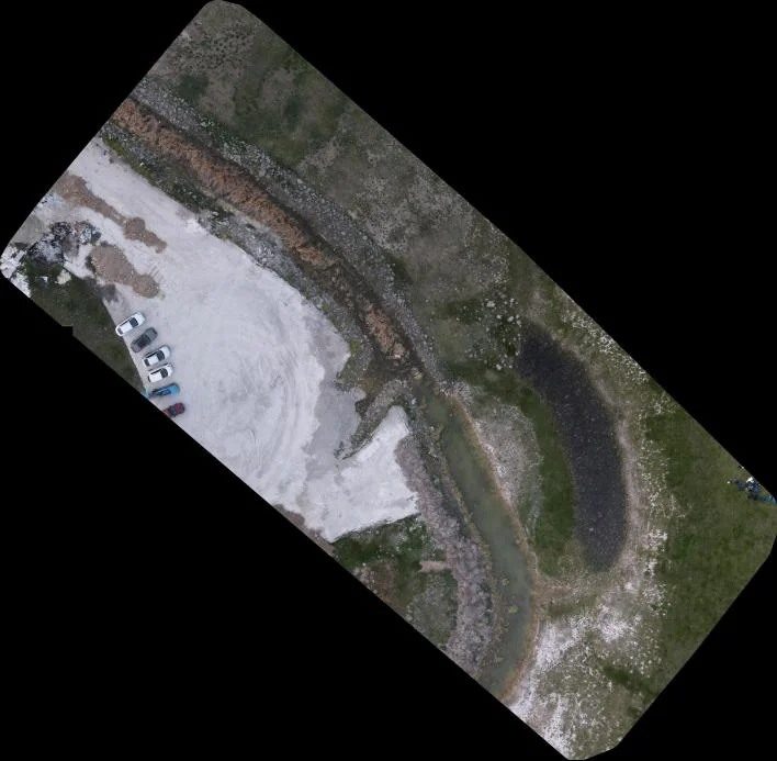
Frame: real output from the project.
Downstream of the map sits the detector, and its numbers explain why the map has to be geometrically honest. We trained YOLOv11m on roughly 15,000 images, tiled to 1280x1280 so the 80 to 120 pixel targets keep enough pixels to learn from. It reached mAP50 of 0.904 and mAP50-95 of 0.691, converging around epoch 33 with early stopping at 48, and inference runs on a Jetson with TensorRT in FP16. A detector at that operating point is rarely the weakest link in the chain; a mosaic with drifting scale would be. The pairing only works because both sides hold up their end.
The failure modes nobody warns you about
- Auto exposure. The sky brightens mid-flight, the camera compensates, and your mosaic becomes a patchwork of brightness steps. Lock exposure if you can.
- Moving objects. A person walking through the overlap zone appears twice as a half-transparent ghost. Blending averages, it does not decide.
- Blending hides geometry errors. Multi-band blending is cosmetic. A seam that looks clean can still sit on top of a misalignment your measurement will find.
- Vibration and rolling shutter. A moving platform skews individual frames slightly. The features still match, the homography absorbs the skew, and the error resurfaces later as a strip that refuses to line up with its neighbour.
- Altitude drift. A few metres of climb between flight lines changes the scale. The matcher tolerates it; the map’s uniform ground resolution does not.
The honest summary: the stitching algorithm was the most reliable part of our mapping pipeline. The flight plan, the exposure settings and the calibration before it decided whether it had anything good to work with.
What I would change next time
Two things. First, treat exposure lock as part of the flight checklist, not as a camera setting you remember on good days. Every mosaic artifact we spent software time on had a cheaper fix available at planning time. Second, keep the model city. It sounds like a toy, but a controlled scene you can re-shoot in minutes is the closest thing a stitching pipeline has to a unit test, and we came back to it every time we touched the code. Field flights validated the system; the model validated the changes.
And a third, smaller one: write the sanity checks down. Straight field lines should stay straight across seams, and a known baseline on the ground should measure the same at both ends of the mosaic. We checked these by eye; a script would have caught regressions faster than we did.