Every tracking pipeline I have built sits on a Kalman filter. The player tracker in our sports video project uses one inside ByteTrack. The target trackers I work on in defence do too. And yet most explanations of it open with five matrices and a page of subscripts, and lose the reader before the idea arrives.
The idea fits in one sentence: you have two guesses about where something is, and you blend them according to how much you trust each one. Everything else is bookkeeping.
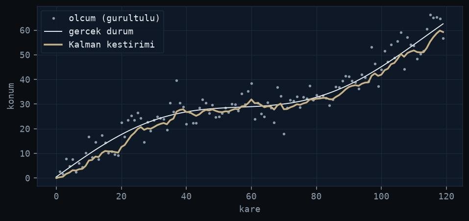 Figure: rendered by me on synthetic data.
Two guesses, one blend
Guess one comes from a motion model. If a player was here last frame and moving at that velocity, physics says they should be roughly there now. Guess two comes from your detector: a bounding box in this frame, with all the jitter detectors produce.
Both guesses are wrong. The question is how wrong, and the filter tracks exactly that: an uncertainty for each guess. The blend weight between them is the Kalman gain. When the motion model has been reliable, the gain leans on the prediction. When the detector is confident and the motion assumption is breaking, it leans on the measurement. That is the whole machine. Predict, correct, repeat.
Predict: uncertainty grows
Between frames, the filter pushes the state forward with the motion model. For box tracking that model is almost always constant velocity: position plus velocity, projected one frame ahead.
The important part is what happens to the uncertainty: it grows. You are extrapolating, and the filter is honest about it. Skip three frames and the predicted position comes with a wide uncertainty band, which is exactly right. A tracker that stays confident while blind is a tracker that steals identities.
Correct: the measurement pulls back
When a detection arrives, the filter pulls the prediction toward it, by the gain amount, and the uncertainty shrinks. A noisy detector pulls weakly. A clean one pulls hard. You never throw either guess away; you average them with weights the filter computed for you.
This is also where the filter earns its money on missed detections. Occlusion, motion blur, a frame where the detector simply fails: the filter keeps predicting, and the track survives. That surviving prediction is what ByteTrack matches low-confidence detections against. Without it, every occlusion is a new identity.
Velocity comes free
A detail that is easy to miss: the state vector is not just position. For box tracking it usually carries position, scale, and their velocities. That means the filter hands you a velocity estimate at every frame, and it is a far better one than anything you could compute yourself by differencing detections. Differentiation amplifies noise. Take the difference of two jittery positions and you get a velocity that swings wildly from frame to frame. The filter’s velocity state, on the other hand, has been smoothed by the same blend of trust that smooths the position. It is the difference between a usable signal and a random number generator.
I did not fully appreciate this until I needed velocity for something real. More on that below.
When the model breaks, that is information
Constant velocity is a lie. Players cut, stop, and accelerate. A ball gets kicked. Every one of those moments violates the motion model, and the filter responds the only way it can: the prediction lands far from the measurement, the gap between them (the innovation, in filter language) spikes, and the estimate lags for a few frames while the filter catches up.
You can treat that lag as a defect and raise Q to reduce it. Or you can notice that the spike itself is a signal. A large innovation means the world just did something your model did not expect. Sometimes that is noise. But when it is consistent over a few frames, it means an actual event happened: a direction change, an acceleration, an impact. The filter is not just an estimator. It is a cheap event detector, if you read its internals instead of only its output.
The matrices, in one paragraph
For completeness: the state vector is what you track, F pushes it forward one step, H maps state to what you can measure, Q says how much you trust the motion model, R says how much you trust the detector. In practice you tune almost nothing but the ratio of Q to R. If your tracks lag behind fast targets, Q is too small: you told the filter the world changes slowly and it believed you. If your tracks jitter along with every noisy box, R is too small. Everything else is usually left at library defaults, and OpenCV ships a perfectly good implementation in cv::KalmanFilter.
Case study: the ball in a single camera feed
The sports video pipeline runs on one fixed wide-angle camera covering the whole pitch. YOLO detects, ByteTrack associates, and a KMeans pass on jersey colors splits the players into teams. Players are the manageable part of that pipeline. The ball is the part that made me respect the Kalman filter all over again.
In a wide shot the ball is a handful of pixels. It moves faster than anything else on the pitch, blurs on every kick, and spends a good share of the match occluded behind legs and bodies. With a single camera there is no second view to rescue you. The detector does what detectors do under those conditions: boxes jitter, vanish for stretches, and occasionally latch onto a sock or a line marking instead. Plot the raw ball detections over time and you get a scatter, not a trajectory.
The filter turns that scatter into a path. Prediction carries the ball through occlusions, and the correct step keeps the noisy measurements from dragging the estimate around. The smoothed trajectory is what gets drawn on the annotated output video, and the difference is visible to anyone: raw detections look like a seismograph, the filtered track looks like physics.
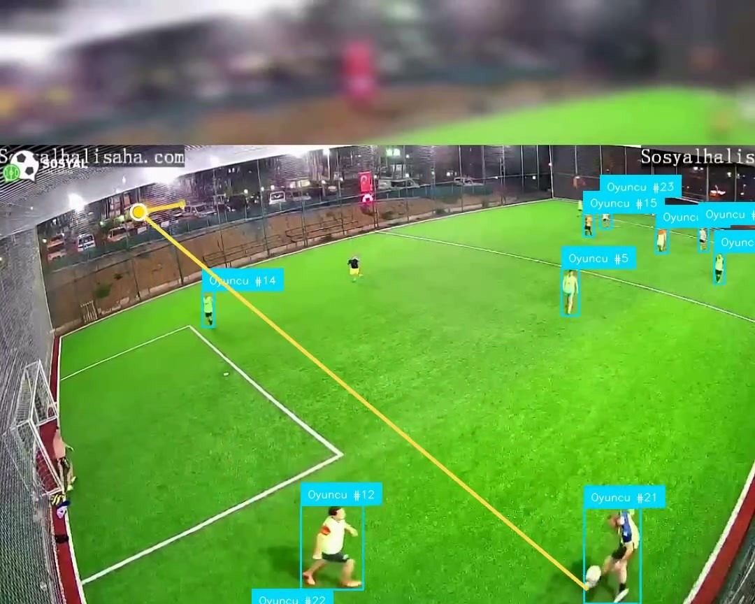 Frame: real output from the project.
The velocity state is where the case pays off. We wanted shot detection, and the honest version of that problem is hard. But a shot has one loud signature: the ball’s speed jumps in an instant. So the pipeline watches the filtered velocity state and flags a sudden jump as a shot candidate. Computing the same thing from raw detections was useless. The frame-to-frame differences were noise, exactly as the section above predicts. The filtered velocity was smooth enough that a genuine kick stood out cleanly. Those events drive the rest of the product: an annotated match video, per-event clips, and a highlight reel, all encoded to H.264 so coaches can play them anywhere.
None of this needed a sophisticated filter. It needed the standard predict and correct loop, a state vector that carries velocity, and the willingness to trust the estimate over the measurement when the measurement is having a bad day.
Where the intuition pays off
On the sports side, players occlude each other constantly and the detector drops boxes every few seconds. On the defence side, the tracking work has to hold a target through frames where the detection channel gives nothing usable. In both cases the Kalman filter is the difference between a track and a pile of disconnected detections.
You do not need to derive it. You need to know which knob to turn when the track lags and which one when it shakes. That is two knobs, not five matrices.